Vineyard Site Suitability Using Multi-criteria Evaluation

“Wine is light held together by water” – Galileo

Preamble….

Beginning in my third year at Brock, I found myself becoming intensely interested in wine and viticulture, so much so that I began revolving my assignments around the industry. Here is a little secret… Believe it or not, doing so made researching much easier through years 3 and 4. Whether physical geography (soil science, climatology), human geography (rural development, tourism, economics) or Geomatics (remote sensing), wine and viticulture allowed me to experience and investigate the interdependencies that make up  so much of what geography is. (And it was FUN!). When I went to Niagara College to do my Post Grad, I decided to continue the Geomatics portion by utilizing GIS in vineyard site suitability analysis.

A Wine Industry Primer…

Before delving into the subject at hand I want to provide some context about the wine industry in Canada and more specifically Ontario. The Grape Growers of Ontario website provides some industry facts including that Ontario is the leading grape producer in Canada representing 85% of the total output while the Niagara Peninsula represents 90% of Ontario’s total output.

As you may or may not know, there are four Designated Viticultural Areas (DVA) in Ontario. These include the Niagara Peninsula, Lake Ontario North Shore, Pelee Island and Prince Edward County (pdf available here). However, other areas of Ontario are building momentum to become DVA’s. The benchmark to achieving this is 125 acres under cultivation (50.5 ha). Ontario South Coast is one of these areas made up of Norfolk County, Elgin County and Middlesex County. Norfolk County was the subject location of this project.

So why Norfolk County??

1. Norfolk County is famous for tobacco production, however with more stringent laws and Provincial/Federal incentives, farmers are looking to move away from tobacco and into other crops. Provision of site suitability maps allows farmers to determine whether their land may be suitable for viticulture.
2. Vineyard and winery developers are seeking to capitalize on the growing popularity of wine tourism.
3. Suitability maps provide generalized topographic information for future agricultural production.
4. Recommendations can be made concerning areas of interest for more localized topographic studies.
5. My climatology professor Dr. Tony Shaw turned me on to Norfolk County through his connection with Burning Kiln winery.

The caveat to all of this however is that site suitability is only one piece of the puzzle. Climatic studies and detailed soil analysis are still needed to come to a final conclusion and ultimately the decision to purchase land and proceed with a vineyard operation.

Site Suitability Parameters:

After an extensive literature review and consultations with the client (Dr. Tony Shaw) the parameters which were utilized for the vineyard site suitability included: slope, aspect, current land use, soil drainage, soil pH, soil depth, depth to ground water, depth to static level ground water and areas of topographic depression.

Some may be wondering why elevation wasn’t considered in this project. The reason for this was because Norfolk County is relatively flat whereby there is only an elevation range of approximately 108 meters between highest and lowest points. It was felt that this would have a negligible impact overall.

Data Collection:

For this particular project, data was acquired through the Brock University Map Library from Land Information Ontario, Ontario Ministry of Agriculture, Food and Rural Affairs (OMAFRA), Ontario Ministry of the Environment (MOE), Ontario Geological Survey and Geobase.

File Preparation for Cumulative Scoring and Pair-wise Comparison Weighted Raster Calculation:

The primary tools used in file preparation for this project were Spatial Analyst (95%) and the ArcHydro Tools 9 extension (5%), used to create the areas of topographic despression file. Based on the DEM cell size of 10m x 10m all subsequent rasters created used this same cell size. The general workflow was the same for each file and consisted of the following:

1. Creation of the files (example – Raster Mosaic for DEM, IDW for groundwater)
2. Reclassification of the files based on optimal parameters (Spatial Analyst Re-class)
3. Conversion of the file to raster (Feature to Raster tool in Spatial Analyst)

This was followed by the actual raster calculations, the buffering of hydrological features (Euclidean Distance Buffer) and road features (Raster Buffer) and the creation of the final suitability maps.

The reclassification scheme of each file consisted of giving a higher re-class value to those attributes that were favourable to higher site suitability. One exception was the reclassification of areas of topographic depression where the lowest re-class value is the most favourable value (in terms of a value that you want to be minimized). This is due to the fact that this value represents smaller areas of topographic depression (vineyard size) where the depression would have the most negative impact on site suitability.

Cumulative Scoring Raster Calculation:

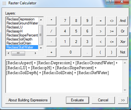
With the nine parameter files created, the cumulative scoring raster calculation could be performed. The summation of these parameters provided a range of values from a lowest of 3 (lowest suitability) to a high of 48 (highest suitability). When the calculation was performed, the results ranged from 10 to 47. One side benefit of raster calculation is that the results can be graphed based on the number of pixels for a particular value. Since these pixels are 100 square meters, total land area can be determined for each score.

The calculation appears in the image below, the results of the raw cumulative scoring appears in the images at the end of this posting.

Pair-wise Comparison Weighted Calculation:

Now be patient… It took me a little while to wrap my head around this concept (mainly because I hadn’t used it before) but also because I was using 9 parameters which became quite daunting. Excel was my friend for sure!

This method employs a ratings scale ranging generally from less important to more important and breaking down further to extremely less or extremely more important. The site suitability project used a 9 point scale but for simplicity sake, I will provide an example using 3 point scale where 1/3 is less important, 1 is equally important and 3 is more important. The parameters are structured in a matrix as illustrated in the example table below.

Pair-wise rankings are established by comparing the parameters between each other. As an example, slope and slope are equally important (1) whereas aspect is more important than slope (3) and drainage is less important than aspect (1/3). These values are summed and then the individual weights are calculated (for slope example 1/2.3333 = 0.4285776. The individual weights are summed together and then averaged (0.4285776+0.4285714+0.4285776 / 3 = 0.428576) to obtain the weights for each parameter. In the above example Slope will represent 42.86% of the weighted calculation.

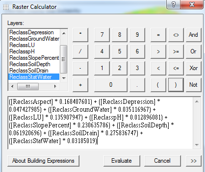
The individual weights are then entered into the raster calculator and multiplied by the parameter raster files. The calculation for all parameters appears on the left. This caluclation provided a range of values between 0.62 and 5.64. To provide the same graphical output, the values need to be reclassed. The maximum number of values which can be assigned using ArcGIS is 32. Using an equal interval classification, the data was reclassed into 32 classes. This allowed the data to be qualitatively compared to the cumulative score data in terms of pixel numbers.

The calculation appears in the image below, the results of the weighted scoring appears in the images at the end of this posting.

The Final Product:

Three different categorization methods were employed for each of the raster calculation results based on the use of Natural Breaks. This provided a much broader overview of the site suitability. A six, four and three class suitability scale using Jenks Natural Breaks was used and compared. The final determination was that a three class ranking provided a much clearer distinction between the rankings of both outputs.

The only thing that needed to be completed was the the buffering of the road network and hydrological features to remove these from the final output as one cannot have a vineyard on the road or in a stream. Again, using raster calculation, these buffered areas were extracted from both the cumulative and wieghted parameter files.

Final results broke down thusly:

Cumulative scoring… 19.26% Low Suitability, 39.98% Moderate Suitability and 40.76% High Suitability

Weighted scoring… 22.12% Low Suitability, 53.47% Moderate Suitabiltiy and 24.40% High Suitability

As the weighted calculation takes into account inter-criteria importance relative to the entire calculation, it is believed that this result provides a more accurate classification of suitability.

Below are the results of each classifcation method. Cumulative on the left and Weighted on the right.

The (In)Consistency Index:

Just when I thought I couldn’t learn anymore during this project, I came upon a method of measuring the potential accuracy (or confidence) in the decision making process of assigning weights to the various criteria in a pair-wise comparison. The (In)Consistency index is often described as a Consistency Index or C.I. This is a measure of the consistency of judgments across all pair-wise comparisons. One reference I found suggests that a tolerance consistency index of 10% be set for comparisons of no more than nine elements. Creating this index also provides a means of determining where the greatest inconsistencies occur so a re-evaluation of a particular comparison can be completed.

When parameters are being weighted within a calculation, creating an (In)Consistency index before completing the raster calculation can only serve to increase the validity of your judgements. The articles are listed below.

Alonso, J.A. and Lamata, M.T. (2006). Consistency in the Analytical Heirarchy Process: A New Approach (pg. 445-459)

Mendoza, G.A. and Macoun, P. (1999). Guidelines for Applying Multi-Criteria Analysis to the Assessment of Criteria and Indicators (this is a Google Books link – Scroll to section 4.2)

Thank you for bearing with me… Had I written a completely detailed account of this project, I’d be upwards of 14000 words (well beyond my posting limit LOL!). If there are any questions please contact me and I will try to answer them as best (and as concisely) as possible.

In the meantime… get ready for the boom of Ontario South Coast Wines. They are well on their way to DVA status… at least in my opinion.

Cheers!

“Wine is bottled poetry” – Robert Louis Stevenson